Preface
Hot Module Replacement (HMR) is a major feature of Webpack. When you modify and save the code, Webpack repackages the code and sends the new module to the browser, which replaces the old module with the new one without refreshing the browser, allowing you to update the application without refreshing the browser.
For example, when developing a web page, if you click a button and a pop-up window appears, but the title of the pop-up window is not aligned, you can modify the CSS style and save it. Without refreshing the browser, the title style changes. It feels like directly modifying the element style in Chrome’s developer tools.
Hot Module Replacement (HMR)
The Hot Module Replacement (HMR) function replaces, adds, or deletes modules during application runtime without reloading the entire page. This significantly speeds up development in the following ways:
Preserve application state lost during a full page reload.
Only update the changed content to save valuable development time.
When CSS/JS changes occur in the source code, they are immediately updated in the browser, which is almost equivalent to directly changing the style in the browser devtools.
Why do we need HMR?
Before the webpack HMR function, there were many live reload tools or libraries, such as live-server. These libraries monitor file changes and notify the browser to refresh the page. So why do we still need HMR? The answer is actually mentioned in the previous text.
Live reload tools cannot save the application state (states). When the page is refreshed, the previous state of the application is lost. In the example mentioned earlier, when you click a button to display a pop-up window, the pop-up window disappears when the browser is refreshed. To restore the previous state, you need to click the button again. However, webapck HMR does not refresh the browser, but replaces the module at runtime, ensuring that the application state is not lost and improving development efficiency.
In the ancient development process, we may need to manually run commands to package the code and then manually refresh the browser page after packaging. All these repetitive work can be automated through the HMR workflow, allowing more energy to be devoted to business instead of wasting time on repetitive work.
HMR is compatible with most front-end frameworks or libraries on the market, such as React Hot Loader, Vue-loader, which can listen to changes in React or Vue components and update the latest components to the browser in real-time. Elm Hot Loader supports the translation and packaging of Elm language code through webpack, and of course, it also implements HMR functionality.
HMR Working Principle Diagram
When I first learned about HMR, I thought it was very magical, and there were always some questions lingering in my mind.
Webpack can package different modules into bundle files or several chunk files, but when I develop with webpack HMR, I did not find the webpack packaged files in my dist directory. Where did they go?
By looking at the package.json file of webpack-dev-server, we know that it depends on the webpack-dev-middleware library. So what role does webpack-dev-middleware play in the HMR process?
During the use of HMR, I know that the browser communicates with webpack-dev-server through websocket, but I did not find new module code in the websocket message. How are the new modules sent to the browser? Why are the new modules not sent to the browser through websocket with the message?
After the browser gets the latest module code, how does HMR replace the old module with the new one? How to handle the dependency relationship between modules during the replacement process?
During the module hot replacement process, is there any fallback mechanism if the replacement module fails?
With these questions in mind, I decided to delve into the webpack source code and find the underlying secrets of HMR.
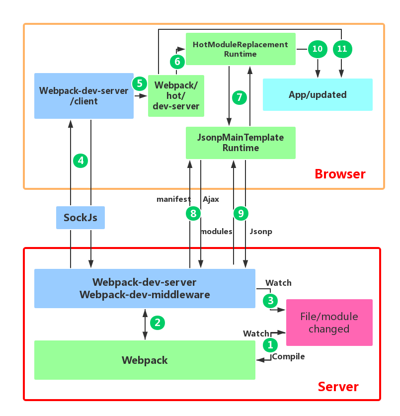
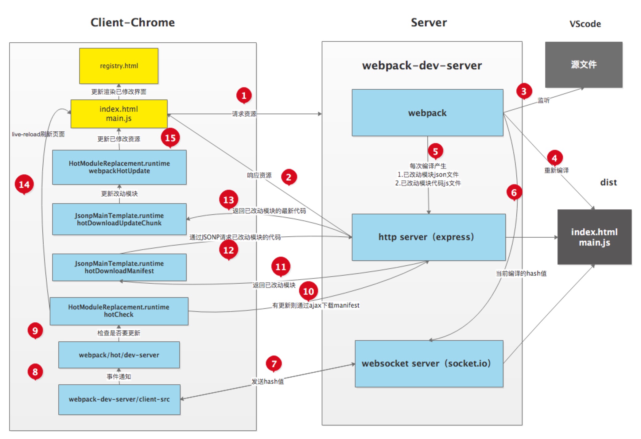
Figure 1: HMR workflow diagram
The above figure is a module hot update process diagram for application development using webpack with webpack-dev-server.
The red box at the bottom of the figure is the server, and the orange box above is the browser.
The green box is the area controlled by the webpack code. The blue box is the area controlled by the webpack-dev-server code. The magenta box is the file system, where file changes occur, and the cyan box is the application itself.
The figure shows a cycle from when we modify the code to when the module hot update is completed. The entire process of HMR is marked by Arabic numerals in dark green.
In the first step, in webpack’s watch mode, when a file in the file system is modified, webpack detects the file change, recompiles and packages the module according to the configuration file, and saves the packaged code in memory as a simple JavaScript object.
The second step is the interface interaction between webpack-dev-server and webpack. In this step, the main interaction is between the dev-server middleware webpack-dev-middleware and webpack. Webpack-dev-middleware calls webpack’s exposed API to monitor code changes and tells webpack to package the code into memory.
The third step is the monitoring of file changes by webpack-dev-server. This step is different from the first step, and it does not monitor code changes and repackage them. When we configure devServer.watchContentBase to true in the configuration file, the server will monitor changes in static files in these configured folders, and notify the browser to perform live reload of the corresponding application after the changes. Note that this is a different concept from HMR.
The fourth step is also the work of the webpack-dev-server code. In this step, the server establishes a websocket long connection between the browser and the server through sockjs (a dependency of webpack-dev-server), and informs the browser of the status information of various stages of webpack compilation and packaging, including the information of Server listening to static file changes in the third step. The browser performs different operations based on these socket messages. Of course, the most important information transmitted by the server is the hash value of the new module. The subsequent steps perform module hot replacement based on this hash value.
The webpack-dev-server/client side cannot request updated code or perform hot module replacement operations, but instead returns these tasks to webpack. The role of webpack/hot/dev-server is to determine whether to refresh the browser or perform module hot updates based on the information passed to it by webpack-dev-server/client and the configuration of dev-server. Of course, if it is only to refresh the browser, there will be no subsequent steps.
HotModuleReplacement.runtime is the hub of client HMR. It receives the hash value of the new module passed to it by the previous step, and sends an Ajax request to the server through JsonpMainTemplate.runtime. The server returns a json that contains the hash values of all modules to be updated. After obtaining the update list, the module requests the latest module code again through jsonp. This is steps 7, 8, and 9 in the above figure.
The tenth step is the key step that determines the success or failure of HMR. In this step, the HotModulePlugin compares the old and new modules and decides whether to update the module. After deciding to update the module, it checks the dependency relationship between the modules and updates the dependency references between the modules while updating the modules.
The last step is to fall back to live reload when HMR fails, that is, to refresh the browser to obtain the latest packaged code.
Simple Example of Using HMR
In the previous section, a HMR workflow diagram was presented to briefly explain the process of module hot updates. However, you may still feel confused, and some of the English terms that appear above may be unfamiliar (these English terms represent code repositories or file modules). Don’t worry, in this section, I will use the simplest and purest example to analyze in detail the specific responsibilities of each library in the HMR process through the webpack and webpack-dev-server source code.
Here, I will use a simple vue example to demonstrate. Here is a link to the repository github.com/ikkkp/webpack-vue-demo
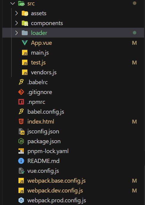
Before starting this example, let me briefly explain the files in this repository. The files in the repository include:
const path = require('path');
const HtmlWebpackPlugin = require('html-webpack-plugin');
const {
    VueLoaderPlugin
} = require('vue-loader');
const webpack = require('webpack'); // 引入 webpack
const AutoImport = require('unplugin-auto-import/webpack')
const Components = require('unplugin-vue-components/webpack')
const {
    ElementPlusResolver
} = require('unplugin-vue-components/resolvers')

/**
* @description
* @version 1.0
* @author Huangzl
* @fileName webpack.base.config.js
* @date 2023/11/10 11:00:59
*/

module.exports = {
    entry: {
        main: './src/main',
        //单页应用开发模式禁用多入口
    },
    resolveLoader: {
        modules: [
            'node_modules',
            path.resolve(__dirname, './src/loader')
        ]
    },
    output: {
        filename: '[id].[fullhash].js', // 使用 [fullhash] 替代 [hash],这是新版本 webpack 的写法
        path: path.join(__dirname, 'dist'),
        publicPath: './'
    },
    module: {
        rules: [{
            test: /\.vue$/,
            loader: 'vue-loader'
        },
        {
            test: /\.css$/,
            use: [
                'style-loader',
                {
                    loader: 'css-loader',
                    options: {
                        importLoaders: 1
                    }
                },
                'postcss-loader'
            ]
        }, {
            test: /\.js$/,
            use: ['babel-loader', {
                loader: 'company-loader',
                options: {
                    sign: 'we-doctor@2021',
                },
            },],
            exclude: /node_modules/,
        },
        {
            test: /\.(ico|png|jpg|gif|svg|eot|woff|woff2|ttf)$/,
            loader: 'file-loader',
            options: {
                name: '[name].[ext]?[hash]'
            }
        },

        ]
    },

    plugins: [
        new HtmlWebpackPlugin({
            template: './public/index.html'
        }),
        new VueLoaderPlugin(),
        new webpack.DefinePlugin({
            BASE_URL: JSON.stringify('./') // 这里定义了 BASE_URL 为根路径 '/'
        }),
        AutoImport({
            resolvers: [ElementPlusResolver()],
        }),
        Components({
            resolvers: [ElementPlusResolver()],
        }),
    ],
    optimization: {
        splitChunks: {
            chunks: 'all', // 只处理异步模块
            maxSize: 20000000, // 设置最大的chunk大小为2MB
        },
    },
};
It is worth mentioning that HotModuleReplacementPlugin is not configured in the above configuration, because when we set devServer.hot to true and add the following script to package.json:
“start”: “webpack-dev-server –hot –open”
After adding the –hot configuration item, devServer will tell webpack to automatically introduce the HotModuleReplacementPlugin plugin, without us having to manually introduce it.
The above is the content of webpack.base.config.js. We will modify the content of App.vue below:
- <div>hello</div> // change the hello string to hello world
+ <div>hello world</div>
Step 1: webpack watches the file system and packages it into memory
webpack-dev-middleware calls webpack’s api to watch the file system. When the hello.js file changes, webpack recompiles and packages the file, then saves it to memory.
// webpack-dev-middleware/lib/Shared.js
if(!options.lazy) {
    var watching = compiler.watch(options.watchOptions, share.handleCompilerCallback);
    context.watching = watching;
}
You may wonder why webpack does not directly package files into the output.path directory. Where do the files go? It turns out that webpack packages the bundle.js file into memory. The reason for not generating files is that accessing code in memory is faster than accessing files in the file system, and it also reduces the overhead of writing code to files. All of this is thanks to memory-fs, a dependency of webpack-dev-middleware. Webpack-dev-middleware replaces the original outputFileSystem of webpack with a MemoryFileSystem instance, so the code is output to memory. The relevant source code of webpack-dev-middleware is as follows: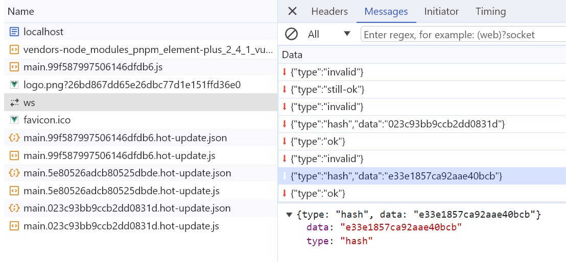
// webpack-dev-middleware/lib/Shared.js
var isMemoryFs = !compiler.compilers && compiler.outputFileSystem instanceof MemoryFileSystem;
if(isMemoryFs) {
    fs = compiler.outputFileSystem;
} else {
    fs = compiler.outputFileSystem = new MemoryFileSystem();
}
First, check whether the current fileSystem is an instance of MemoryFileSystem. If not, replace the outputFileSystem before the compiler with an instance of MemoryFileSystem. This way, the code of the bundle.js file is saved as a simple JavaScript object in memory. When the browser requests the bundle.js file, devServer directly retrieves the JavaScript object saved above from memory and returns it to the browser.
Step 2: devServer notifies the browser that the file has changed
In this stage, sockjs is the bridge between the server and the browser. When devServer is started, sockjs establishes a WebSocket long connection between the server and the browser to inform the browser of the various stages of webpack compilation and packaging. The key step is still webpack-dev-server calling the webpack API to listen for the done event of the compile. After the compile is completed, webpack-dev-server sends the hash value of the newly compiled and packaged module to the browser through the _sendStatus method.
// webpack-dev-server/lib/Server.js
compiler.plugin('done', (stats) => {
  // stats.hash 是最新打包文件的 hash 值
  this._sendStats(this.sockets, stats.toJson(clientStats));
  this._stats = stats;
});
...
Server.prototype._sendStats = function (sockets, stats, force) {
  if (!force && stats &&
  (!stats.errors || stats.errors.length === 0) && stats.assets &&
  stats.assets.every(asset => !asset.emitted)
  ) { return this.sockWrite(sockets, 'still-ok'); }
  // 调用 sockWrite 方法将 hash 值通过 websocket 发送到浏览器端
  this.sockWrite(sockets, 'hash', stats.hash);
  if (stats.errors.length > 0) { this.sockWrite(sockets, 'errors', stats.errors); }
  else if (stats.warnings.length > 0) { this.sockWrite(sockets, 'warnings', stats.warnings); }      else { this.sockWrite(sockets, 'ok'); }
};
Step 3: webpack-dev-server/client responds to server messages
You may wonder how the code in bundle.js receives websocket messages since you did not add any code to receive websocket messages in your business code or add a new entry file in the entry property of webpack.config.js. It turns out that webpack-dev-server modifies the entry property in webpack configuration and adds webpack-dev-client code to it. This way, the code in bundle.js will have the code to receive websocket messages.
When webpack-dev-server/client receives a hash message, it temporarily stores the hash value. When it receives an ok message, it performs a reload operation on the application. The hash message is received before the ok message.
In the reload operation, webpack-dev-server/client stores the hash value in the currentHash variable. When it receives an ok message, it reloads the App. If module hot updates are configured, it calls webpack/hot/emitter to send the latest hash value to webpack and then hands over control to the webpack client code. If module hot updates are not configured, it directly calls the location.reload method to refresh the page.
Step 4: webpack receives the latest hash value, verifies it, and requests module code
In this step, three modules (three files, with the English names corresponding to the file paths) in webpack work together. First, webpack/hot/dev-server (referred to as dev-server) listens for the webpackHotUpdate message sent by webpack-dev-server/client in step 3. It calls the check method in webpack/lib/HotModuleReplacement.runtime (referred to as HMR runtime) to check for new updates. In the check process, it uses two methods in webpack/lib/JsonpMainTemplate.runtime (referred to as jsonp runtime): hotDownloadUpdateChunk and hotDownloadManifest. The second method calls AJAX to request whether there are updated files from the server. If there are, it returns the list of updated files to the browser. The first method requests the latest module code through jsonp and returns the code to HMR runtime. HMR runtime further processes the returned new module code, which may involve refreshing the page or hot updating the module.
It is worth noting that both requests use the file name concatenated with the previous hash value. The hotDownloadManifest method returns the latest hash value, and the hotDownloadUpdateChunk method returns the code block corresponding to the latest hash value. Then, the new code block is returned to HMR runtime for module hot updating.
Step 5: HotModuleReplacement.runtime hot updates the module
This step is the key step of the entire module hot updating (HMR), and all module hot updates occur in the hotApply method of HMR runtime.
// webpack/lib/HotModuleReplacement.runtime
function hotApply() {
    // ...
    var idx;
    var queue = outdatedModules.slice();
    while(queue.length > 0) {
        moduleId = queue.pop();
        module = installedModules[moduleId];
        // ...
        // remove module from cache
        delete installedModules[moduleId];
        // when disposing there is no need to call dispose handler
        delete outdatedDependencies[moduleId];
        // remove "parents" references from all children
        for(j = 0; j < module.children.length; j++) {
            var child = installedModules[module.children[j]];
            if(!child) continue;
            idx = child.parents.indexOf(moduleId);
            if(idx >= 0) {
                child.parents.splice(idx, 1);
            }
        }
    }
    // ...
    // insert new code
    for(moduleId in appliedUpdate) {
        if(Object.prototype.hasOwnProperty.call(appliedUpdate, moduleId)) {
            modules[moduleId] = appliedUpdate[moduleId];
        }
    }
    // ...
}
From the hotApply method above, it can be seen that module hot replacement mainly consists of three stages. The first stage is to find outdatedModules and outdatedDependencies. I did not include this part of the code here, but if you are interested, you can read the source code yourself. The second stage is to delete expired modules and dependencies from the cache, as follows:
delete installedModules[moduleId];
delete outdatedDependencies[moduleId];
The third stage is to add the new module to the modules object. The next time the __webpack_require__ method (the require method rewritten by webpack) is called, the new module code will be obtained.
For error handling during module hot updates, if an error occurs during the hot update process, the hot update will fall back to refreshing the browser. This part of the code is in the dev-server code, and the brief code is as follows:
module.hot.check(true).then(function(updatedModules) {
    if(!updatedModules) {
        return window.location.reload();
    }
    // ...
}).catch(function(err) {
    var status = module.hot.status();
    if(["abort", "fail"].indexOf(status) >= 0) {
        window.location.reload();
    }
});
dev-server first verifies if there are any updates, and if there are no code updates, it reloads the browser. If an abort or fail error occurs during the hotApply process, the browser is also reloaded.